Principal Component Analysis on the US Yield Curve
Introduction
Principal Component Analysis (PCA) is often used to reduce data dimensionality in machine learning. A classical example in finance is applying PCA on the yield curve, which loosely describes the rate of return of government bonds at different maturities.
In the past, I have learned from various lectures and reading materials that:
The first principal component describes a parallel shift of the yield curve,
The second principal component describes its tilt (i.e. first-order derivative), and
The third principal component describes its curvature (i.e. second-order derivative).
I have always taken the points above as given, but now I would like to actually observe this from real data. Besides, I would also like to implement PCA step by step to brush up my understanding of the topic.
Overview of Data
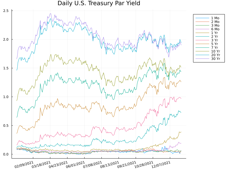
The daily US treasury par yield curve rates can be downloaded from the US Department of the Treasury. The raw data is a csv file that contains the yield rates for different maturities observed on each of the 251 trading days in 2021.
We can plot the rates by different maturities (or terms) against the trading dates, as shown below. In this plot, each line represents the dynamic change of the yield rate for bonds with the a particular maturity. It is clear that rates at different terms are highly correlated, but the correlation is not perfect. This type of correlated data are suitable for applying PCA for dimension reduction.
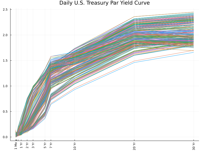
Another way to visualize the data is to plot the yield curve with all maturities for each trading day, as shown below. In this case, each line represents the observation of yield rates of all maturities on a particular trading day. At first sight, we observe a lot of parallel lines, especially for longer maturities such as 5 years and beyond.
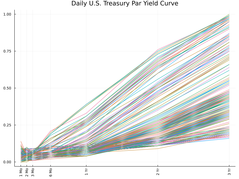
We can also zoom in on the rates for shorter maturities. They are not as parallel as longer-term rates. Rather, the 1-year, 2-year and 3-year rates are typically more spreadout than those with maturities less than 1 year.
PCA Implementation
The details of implementing PCA have been covered by many excellent textbooks and online tutorials, such as here and here. I will not bother with repeating the exact same procedures, but only note down the following key steps for this particular application in analyzing the yield curve:
Instead of looking at the raw data, we are more interested in the daily changes in yield rates, which results in 250 rows of data.
Normalization is important. The data will be centered by mean and further divided by their standard deviation.
Results and Interpretation
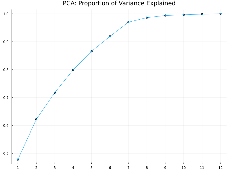
Proportion of Variance Explained
Out of all twelve components, the first four explain roughly 80% of the total variance, as shown below. This is typically a reasonable representation of the original data, considering the dimension is reduced by 67%.
PCA Loadings
The PC loadings (or eigenvectors of the covariance matrix) demonstrate how each PC differentiates the data points. Below we plot the PC loadings for the first four PC's.
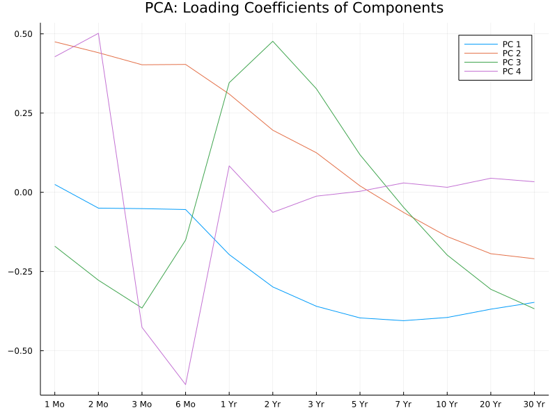
Note that the absolute signs of the PC loadings do not matter, but rather their relative magnitude. With this in mind, we can make the following interpretations of the PC's:
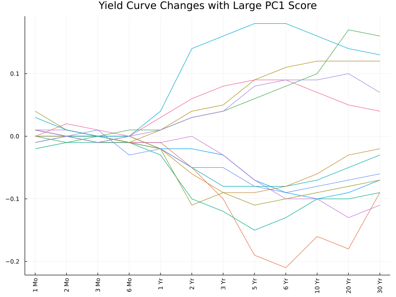
The first PC mainly describes parallel shifts of the yield curve, more specifically shifts in longer-term rates (longer than 2 years).
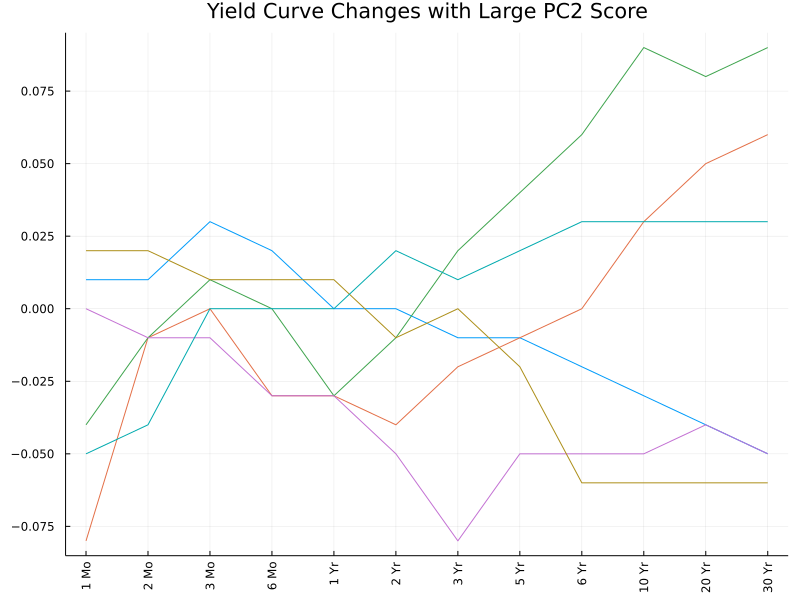
The second PC describes the simultaneous movements of short-term and long-term rates in opposite directions.
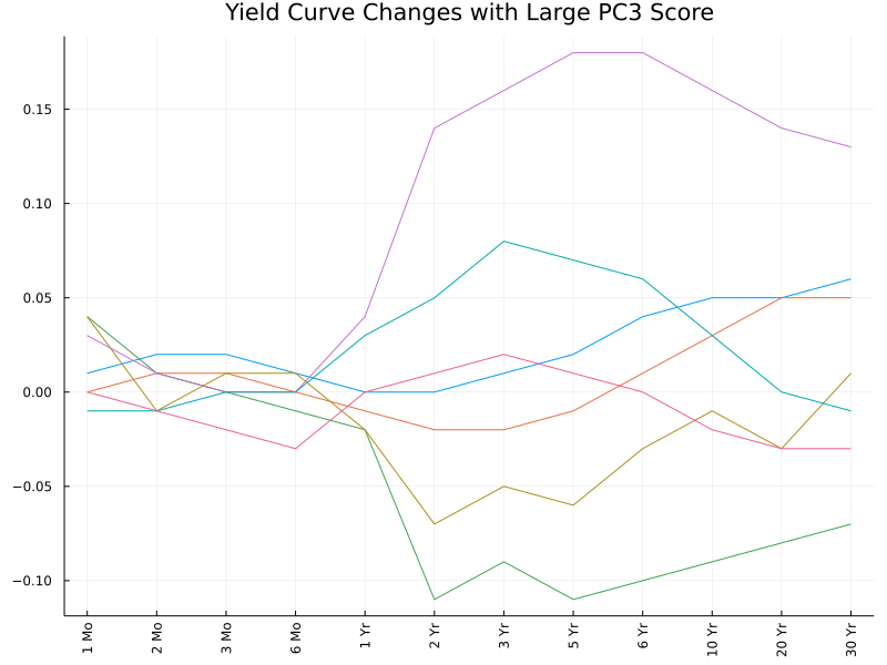
The third PC describes curvatures of the yield curve, in particular, contrasting the opposite movements of 1- to 5-year yield rates against the rest.
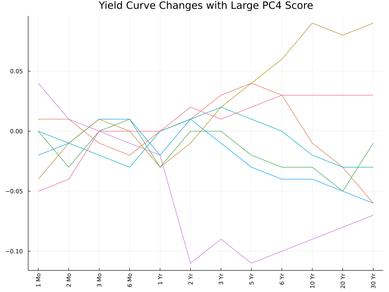
The fourth PC seems to contrast opposite movements between 1- and 2-month rates agianst 3- and 6-month rates.
These interpretations can also be confirmed (to some extent) by the following plots. We pick out observations with the highest PC scores (in absolute values) and plot the corresponding changes in the yield curve. The first two plots are somewhat easy to interpret, while the remaining appear more messy and hard to interpret.
Conclusion
In short, this has been a good exercise for me to revisit some key concepts and steps in PCA. The numerical results from this particular dataset (kind of) align with what I have previously learned about PCA, although not perfectly due to various reasons such as the size and randomness of the dataset, etc.
Website built with Franklin.jl and the Julia programming language,
plus some help from LeXtudio.